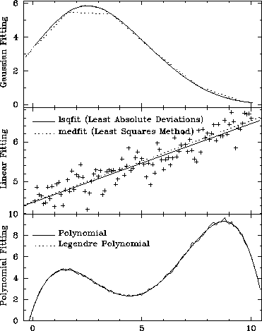
Figure E.9: A plot showing different ways to fit data.


define display     # $1 = panel number; $2 = data file; $3 = Fit type.
color 1            # Reset color index.
panel 1 -3 -$1     # Set the selected panel.
data $2            # Open the data file.
xcolumn 2
ycolumn 3
ecolumn 4
ylabel \fr $3 Fitting
end

viewport 0.2 0.8 0.2 0.8 # Set the viewport scale.
font 2             # Choose a nice font.
expand 1.2         # Choose a nice expansion.
display 1 gauss.dat Gaussian # Read data containing two gaussians.
limits             # Autoscale the limits.
connect            # Draw the data.
box bcst bncstv    # Draw the box (no X numbers).
fit gauss 2  4.5 2.2 2.8  2.5 4.9 2.8 # Fit 2 gaussians.
lstyle 4           # Select a dashed line style.
color 3            # Set color to green.
plotfit x1 x2 0.5  # Plot the fit at high resolution.
color 4            # Set color to blue.
plotfit x1 x2 2.0  # Plot the fit at coarse resolution.
lstyle 1           # Reset line style to solid.
range 6 10         # Limit the range in the X direction.
fit gauss 2  4.5 2.2 2.8  2.5 4.9 2.8 # Fit 2 gaussians.
range 0 0          # Reset the range to the full X-axis.
color 2            # Set color to red.
plotfit 6 10       # Plot the fit for the limited range.

display 2 line.dat Linear # Read data scattered linearly.
limits x1 x2 0 0   # Retain X limits; autoscale Y limits.
symbol 2           # Select the '+' symbol.
points             # Display data as points.
box bcst bncstv    # Draw the box (no X numbers).
fit lsqfit         # Fit via Least Squares method.
color 3            # Set color to green.
plotfit            # Plot the lsqfit solution.
move 0 6.5         # Draw a line for...
draw 1 6.5         # ... the fit legend.
label \fr lsqfit (Least Absolute Deviations)
fit medfit         # Fit via Least Absolute Deviations.
color 4            # Set color to blue.
lstyle 4           # Select a dashed line style.
plotfit            # Plot the medfit solution.
move 0 6.2         # Draw a line for...
draw 1 6.2         # ... the fit legend.
label \fr medfit (Least Squares Method)
lstyle 1           # Reset line style to solid.
color 1            # Reset color index.

display 3 poly.dat Polynomial # Read data containing a polynomial.
limits x1 x2 0 10  # Retain X limits; autoscale Y limits.
connect            # Draw the data.
box bcnst bncstv   # Draw the box (with X numbers).
fit polynomial 5   # Fit a simple polynomial of order 4.
color 3            # Set color to green.
plotfit            # Plot the polynomial solution.
move 0 8           # Draw a line for...
draw 1 8           # ... the fit legend.
label \fr Polynomial
fit legendre 5     # Fit a Legendre polynomial of order 4.
color 4            # Set color to blue.
lstyle 4           # Select a dashed line style.
plotfit            # Plot the Legendre solution.
move 0 7           # Draw a line for...
draw 1 7           # ... the fit legend.
label \fr Legendre Polynomial
lstyle 1           # Reset line style to solid.
color 1            # Reset color index.

Figure E.9: A plot showing different ways to fit data.